Model Explanation
NSCD
Our Non Smooth Contact Dynamics grain solver
VANS
Our Volume Averaged Navier Stokes fluid solver
Meshing methods
PFEM and other mesh-based remeshing strategies
It is important to note that within the granular flows field there are many different types of applications, which can be computed in a variety of ways. The model you use may depend on the quantity you are trying to observe. In this section, we briefly outline the possibilities offered by the MigFlow software — and the choices behind them.
Immersed granular flows are also encountered in geology, e.g. mud volcanoes, hydrothermal vents, etc. Natural geometries in which fluid-grain mixtures flow can be just as complex as the industrial geometries in applications like gas cyclone separators, ploughshare mixers, semi-autogenous grinding mills, tower mills, etc. The Finite Element Method is easily applicable to complex geometries thanks to the use of irregular grids.
MigFlow represents the grains individually with Non-Smooth Contact Dynamics (NSCD): a hard-sphere approach that never lets grains overlap and solves directly for the contact impulses that prevent it, buying a larger, more robust time step and strict volume conservation of the packing. The details of this method are covered on the NSCD axis.
The fluid side offers a second, largely independent choice: whether to resolve the flow around every grain. Resolved approaches capture the boundary layer around each particle directly, at a cost that grows steeply with the number of grains. Unresolved approaches instead average the fluid equations over a control volume spanning many grains, reintroducing their influence through a closure force; this is the Volume-Averaged Navier–Stokes (VANS) formulation MigFlow builds on, detailed on the VANS axis. What sets MigFlow's implementation apart is that this formulation is no longer tied to one end of that spectrum: an overlap-wise grain representation and a semi-implicit coupling scheme let the same numerical scheme move continuously from unresolved — a mesh far coarser than a grain — to semi-resolved — a mesh comparable to a grain — without changing the underlying equations or requiring an artificial smoothing kernel.
This scale flexibility is the foundation the rest of the framework builds on. Heat transfer and phase change (see Non-isothermal flows) extend the same fluid–grain coupling to thermal exchange, while the Particle Finite Element Method (see Meshing methods) extends it to domains whose geometry itself evolves — free surfaces, large deformations, and the real-world events explored throughout this site, from a digging droplet to a landslide-generated tsunami.
Grains Representation
Fine Scale Model for the Grains
The main attribute of the solid granular phase is its volume conservation. In our numerical description, grains are treated as rigid bodies: they do not deform, and they are never allowed to interpenetrate. Plus, the geometrical microscopic configuration of the granular matrix greatly affects the macroscopic behaviour of the medium: a few clogged grains can lock the surrounding contact network in place and prevent the whole material from flowing — a phenomenon known as jamming. The granular phase is thus solved with a Discrete Element Method that tracks the positions and velocities of the grains in a Lagrangian way.
Friction, Cohesion and so on…
The MigFlow software can take into account friction between the grains in various ways. First, the free velocities of the grains are computed from Newton’s second law, given the external forces acting on the grains such as gravity or drag from the fluid. Second, the collisions between the grains are solved using the Nonsmooth Contact Dynamics. This time-stepping method corrects iteratively the free velocities of the grains, obtained by applying external forces, to compute a set of velocities giving after displacement of the grains a stationary state without intersection. This implicit method solves all the contacts active over the time step together, using a Non-Linear Gauss–Seidel iterative procedure: each contact is revisited in turn, over and over, until the whole system converges. The MigFlow software makes use of a queue to speed up this iterative process, prioritising contacts that have not yet converged. The resolution of a contact is based on a momentum balance so that grain interpenetration is prevented. Friction is taken into account with a Coulomb law. This approach allows for a large time step while maintaining strict volume conservation of the packing. With this resolution of the granular phase, it is possible to obtain the force network between the grains as well as the stress tensor inside them.
The scontact Local Solver
Its own frictional contacts solver, scontact, can solve friction in both 2D and 3D for spherical grains, considering that they can rotate or not. This local solver takes advantage of the sphericity of the particles to be very fast and efficient. The forces exerted by the grains on the domain boundaries can be computed, as well as the stress tensor inside the grains. It is also possible to set periodic conditions at the boundaries. Finally, scontact allows to fix some grains so that they act like a boundary, enabling the simulation of a granular flow through a fixed porous media for example.
LMGC90 Software Compatibility
Another possibility is to use LMGC90 Software (for installation we recommend to follow the instructions on their website), which is compatible with the fluid solver of MigFlow. This way, more complex contact laws and particle shapes can be taken into account. Note that the fluid solver will always consider spherical shapes for the grains.
Relevant Grain Testcases
- Rotating Mill Particle Simulation presents the mixing of grains with different radii in a rotating drum using LMGC90 or scontact to take into account the impact of the friction on the mixing efficiency.
- Bidimensional shear of a dry granular material presents a simulation showing how to use the available methods to analyze contact dynamics, force networks, and friction effects without fluid involvement.
Fluid Representation
A Multiscale Model for the Fluid
Industries often require fast software to calibrate their processes. The model we propose represents the fluid on a mesh whose resolution is chosen independently of the grain size, rather than fixing it once and for all — from a coarse mesh homogenising a dense packing to a fine mesh resolving individual grains. The flow dynamics in the space between the grains is computed from averaged Navier-Stokes equations, and the local fluid volume fraction is used to average pointwise field values into a continuous representation of the mixture flow.
Upper Figures show the discrete grains, while the lower Figures show the continuous representation of the fluid volume fraction
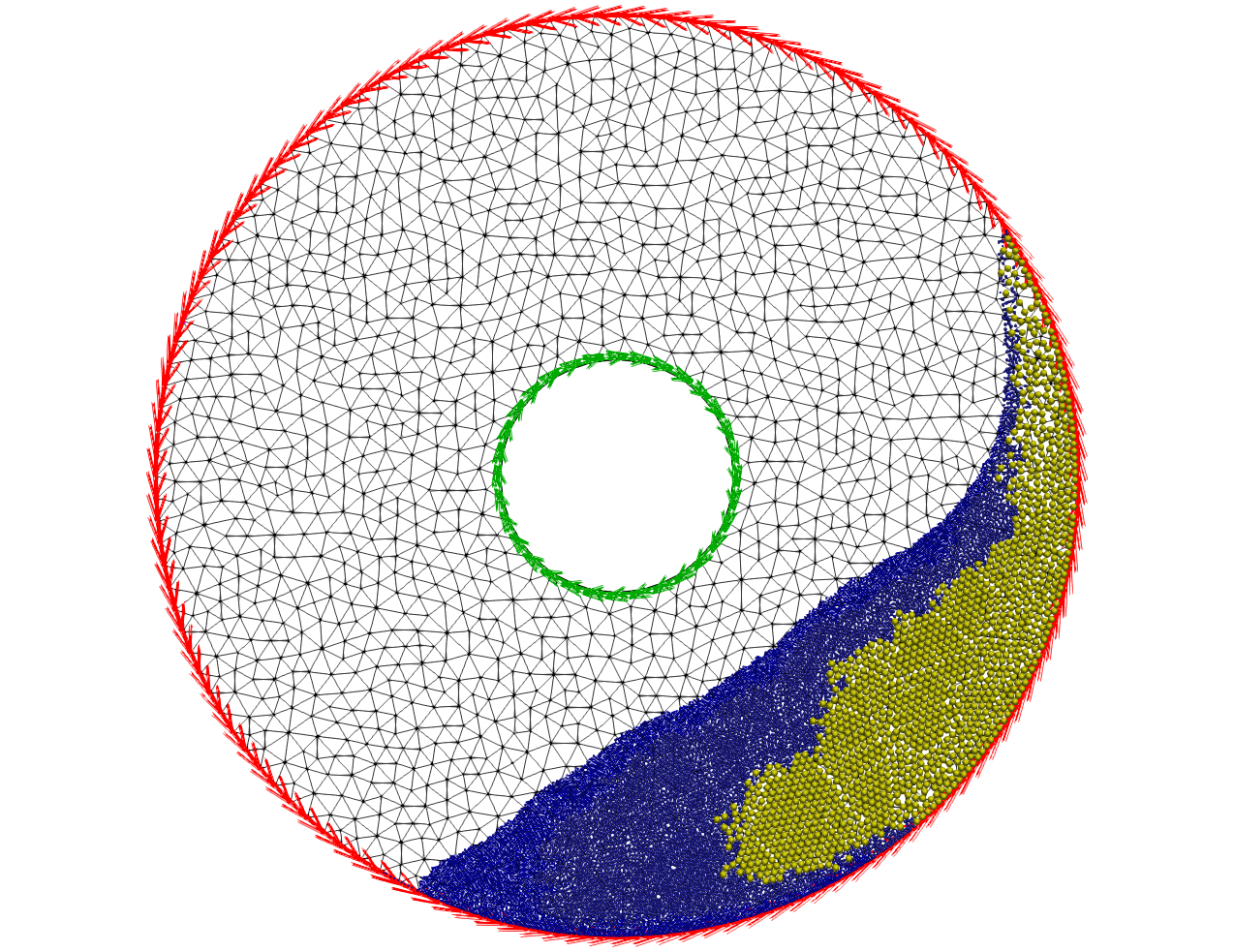
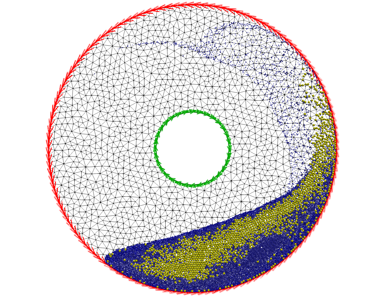
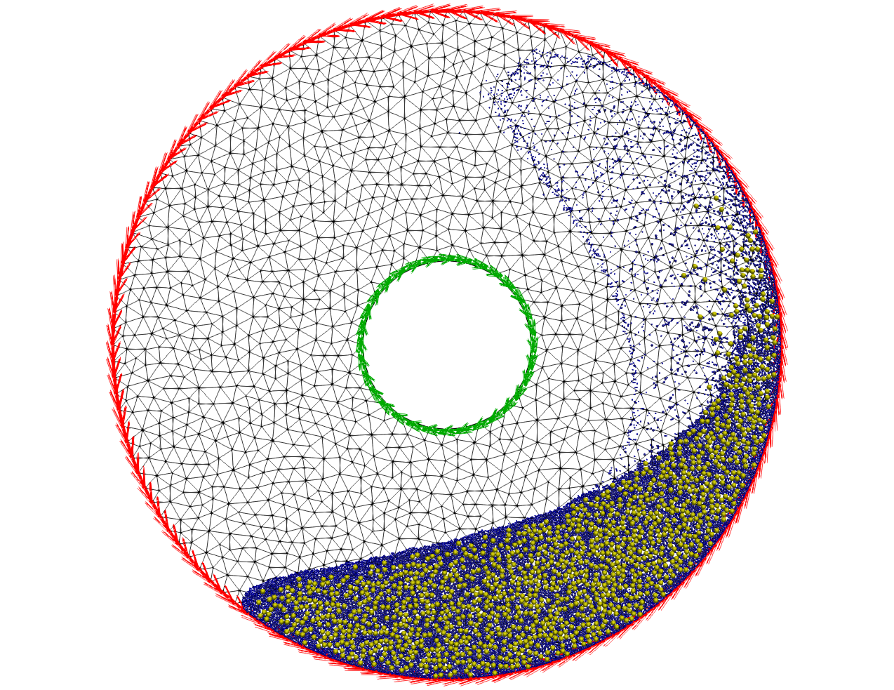
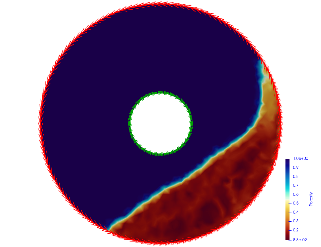
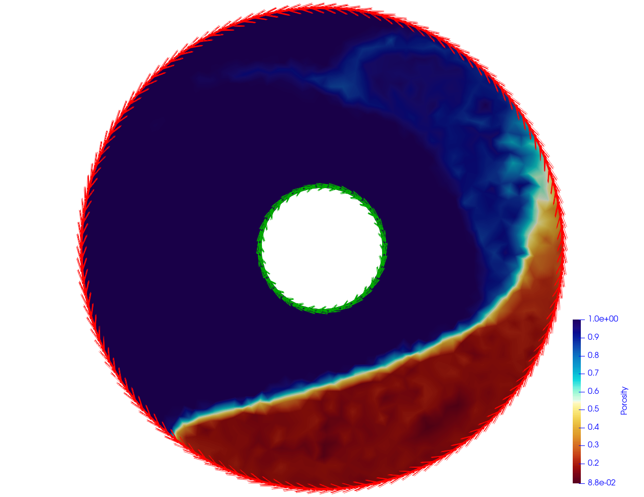
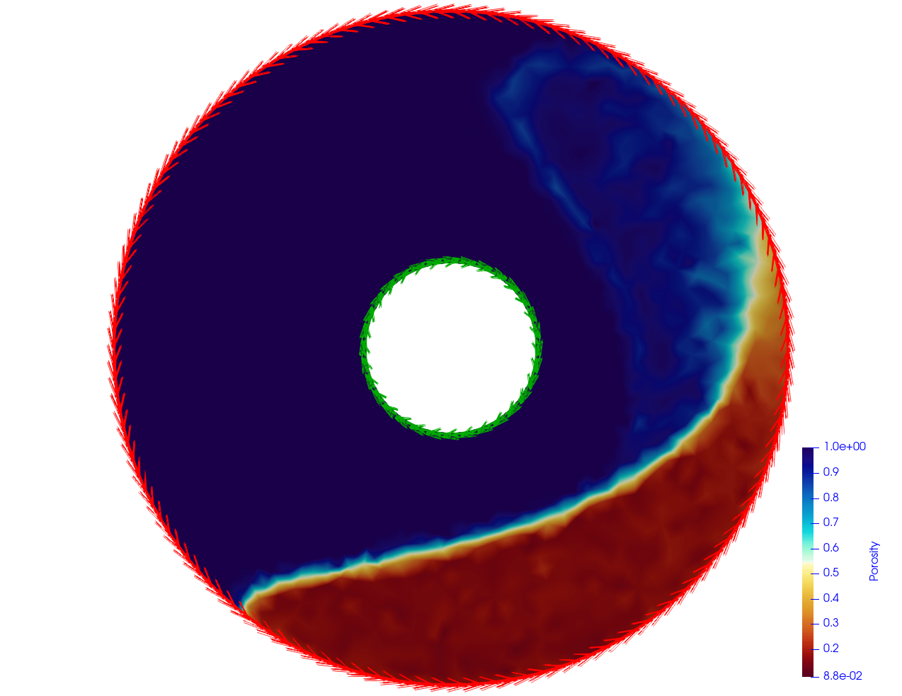
The continuous representation of the mixture gives the possibility to cover the entire domain with a continuous mesh, preventing the numerical cost of a mesh reconstruction on the fluid phase at each grain displacement or the use of a penalty method. The transition between the pure fluid regime and the granular medium regime is covered by the averaging process in the modified Navier-Stokes equations. The average variables taking into account the fluid volume fraction enable a continuous transition between the two flow regimes.
Adaptive Mesh
MigFlow is based on a Computational Fluid Dynamics–Discrete Element Method model that spans unresolved, semi-resolved, and fully resolved regimes within the same numerical scheme. The discretisation method we choose for the CFD part is the Finite Element Method. On the one hand, unstructured grids offer a great flexibility to represent complex geometries with which grains interact. On the other hand, it is easy to adapt the mesh in order to refine it around the area of interest to accurately capture flow fields during the grains motion.
fluid.adapt_mesh(Max. element size, Min. element size, Total number of elements, a, b)The arguments a and b in the adapt_mesh function are optional. These parameters are used to weigh the maximum and minimum gradient used to compute the new mesh size at each node of the old mesh. For more information on the refinement formula see: Constant, M., Dubois, F., Lambrechts, J. and Legat, V. (2018). Implementation of an unresolved stabilised FEM-DEM model to solve immersed granular flows. Computational Particle Mechanics. doi:10.1007/s40571-018-0209-4.
Adaptive Mesh Testcases
- Bidimensional fall of a single cloud made of particles in a viscous fluid presents the fall of a cloud made of grains in a viscous fluid and makes use of this feature to refine the mesh around the cloud area during the fall. This way, it is possible to highly fasten the computation because the area of interest (i.e. the cloud) is small compared with the entire computational domain.
- Granular Column Collapse in Fluid presents the fall of a granular column immersed in soft water.
Advanced Computational Methods
Two Fluids + Grains
To consider two continuous phases, an advective equation for the concentration is added to the standard Navier-Stokes equations. See the following example to run test cases with two different continuous phases:
• Water–Salt Water Avalanche presents the fall of a granular column immersed in sea water in a 2D domain filled with soft water.
Arbitrary Eulerian-Lagrangian (ALE) method & Free Surface
The MigFlow software can take into account mesh deformation using the Arbitrary Eulerian-Lagrangian (ALE) framework. The user has to provide the mesh velocity and update the mesh coordinates. This feature can be used to simulate free-surface, and underpins the more specialised meshing strategies developed within the group — the Particle Finite Element Method (PFEM), which rebuilds the domain from the particle positions at every time step, and X-Mesh, which deforms a fixed-connectivity mesh to track an interface without remeshing at all (see Meshing methods):
- 2D Poiseuille flow with PFEM serves as a core formulation reference for validation.
- Die Swell of a Newtonian Fluid presents the swelling of a flow past a die in 2D.
Periodic Conditions & Mesh Constraints
Periodic conditions are available. The periodicity transformations are deduced from the mesh file. For the fluid phase, two points which are periodic will have the same degree of freedom. As for the solid phase, a ghost particle is created if a particle is close to a periodic boundary. Similarly to the fluid approach, the ghost particle is only a pointer to its parent particle. Multiple examples of this feature can be explored via Fluid Transport in a 2D Periodic Channel.
The configuration information is directly extracted from the mesh file. Therefore, to apply a boundary condition, the .geo file has to contain this information. No boundary conditions have to be imposed on the periodic boundaries. Be careful about the line orientation while specifying periodicity in your .geo file. You can review this configuration standard within 2D Poiseuille flows.
Closure Terms
Momentum balance
The connection between the fine-scale representation of the grains and the coarse-scale representation of the fluid flow requires an empirical force to model the momentum transfer between the discrete and the continuous phases. This closure term is a drag force accounting for the relative velocity between the grains and the fluid, the presence of neighbouring grains, and a handful of other physical parameters.
In the continuous representation of the mixture, this fluid-grains interaction force is applied as a source term, which can become dominant depending on the flow regime. A semi-implicit scheme is used to stabilise the resolution of the averaged Navier-Stokes equations, allowing sufficiently large time steps to take full advantage of the implicit formulation. These empirical closure terms have been tested and found able to reproduce fine-scale features of immersed granular flows.
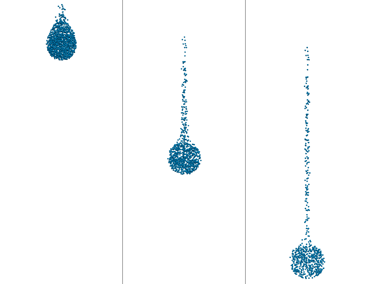
Macro-scale visualisation showcasing the empirical momentum-transfer closure validated on a Stokes cloud model