Research Axis - Meshing methods

The Meshing methods group develops and maintains the mesh-based backbone shared by MigFlow's fluid solvers: the strategies used to track a deforming domain, its free surface, and its interfaces over time without letting element quality degrade. This axis centres on the Particle Finite Element Method (PFEM), which remeshes the domain at every time step from the advected node positions, but is not limited to it — it also covers complementary or alternative meshing strategies developed within the group, such as X-Mesh and the Tempered Finite Element Method (TFEM). The two are directly connected: X-Mesh tracks an interface by handing it over from one layer of mesh nodes to the next, which can leave behind bands of very thin, nearly degenerate elements; TFEM is precisely what makes computing on those bands tractable, by locally and provably relaxing the finite element formulation just enough to avoid the locking that would otherwise break convergence. The common thread across the axis is making large deformations, free-surface tracking, and multi-phase interfaces tractable at the mesh level, so that the physics solvers built on top (VANS, NSCD) can be reused across configurations regardless of which meshing strategy is driving them.

Key Concepts & Methodology

ALE: Tracking an Interface by Moving With It

The simplest way to track a moving interface is to move the mesh with it: Arbitrary Lagrangian–Eulerian (ALE) advects the mesh at the interface velocity and solves the flow in that moving frame,

$$ \frac{\mathrm{d}\bullet}{\mathrm{d}t}\bigg|_{\mathbf{x}} = \frac{\partial\bullet}{\partial t} + (\mathbf{u}-\mathbf{u}_{\mathrm{mesh}})\cdot\nabla\bullet, \qquad \mathbf{u}_{\mathrm{mesh}} = \frac{\mathbf{x}^n-\mathbf{x}^{n-1}}{\Delta t}. $$

Simple and accurate, with excellent conservation — but it only survives moderate deformation: past a point, the mesh itself must be rebuilt or radically changed.

PFEM: Rebuilding the Mesh Every Step

PFEM solves ALE's limit head-on: instead of deforming one mesh, it rebuilds the whole domain from the particle positions at every time step, via a Delaunay triangulation filtered by the α-shape criterion,

$$ R_e < \alpha \cdot h(\mathbf{x}). $$

Elements whose circumradius $R_e$ exceeds this bound are discarded, recovering a sharp, topology-changing free surface. This handles arbitrarily large deformation, at the cost of remeshing — and re-interpolating the solution — every single step.

Coupled two-way to NSCD, this same PFEM mesh also carries a granular phase: walls are never explicitly meshed but detected geometrically (via a quadtree) so boundary conditions still apply cleanly to a domain that is rebuilt every step, and the fluid–grain drag is made stable by a semi-implicit prediction of each grain's velocity rather than a fully explicit one. This PFEM–DEM formulation (Leyssens et al., 2025) is what drives the fluid–grain simulations further down this page.

X-Mesh: Deforming Instead of Remeshing

X-Mesh keeps PFEM's large-deformation, topology-change capability without ever remeshing: connectivity stays fixed, and only node positions move, collapsing elements to zero measure to relay the interface from node to node. Because nodes sit exactly on the interface at all times, conditions like the surface-tension pressure jump can be imposed exactly rather than smeared over an element,

$$ [p] = -\sigma\kappa, $$

at the cost of deliberately producing degenerate elements (needles, harmless; caps, dangerous in bands).

TFEM: Making Degenerate Elements Safe

Both PFEM and X-Mesh can leave behind degenerate elements — caps, slivers — that lock the finite element solution once they chain into bands. TFEM fixes this with one local change: flooring the element mapping's Jacobian to soften the diffusion coefficient just on the degenerate region,

$$ \int_\Omega d(\mathbf{x})\,\nabla u_h\cdot\nabla v_h\,\mathrm{d}x = \int_\Omega f v_h\,\mathrm{d}x, \qquad J_{\min}\sim h^{d+1}, $$

recovering the full convergence rate everywhere else — the piece that lets PFEM's and X-Mesh's degenerate elements be computed on safely.

Featured Simulation

Fluid-Grain Mixing in a Rotating Mill

Supplementary documentation

Leyssens et al. (2025), J. Comput. Phys.

Simulated by

Simulation Overview

Fluid and grains are mixed together inside a rotating drum, with the same two-way PFEM–DEM coupling used throughout this axis: the fluid's free surface is rebuilt every step by PFEM while the grains are resolved individually by NSCD and fed back into the fluid through the VANS-family projection. Rather than a landslide-style benchmark, this case illustrates the versatility of the coupling itself — deforming free surfaces, fluid–grain interaction, and a continuously moving boundary (the rotating mill wall) all handled at once, as showcased in Leyssens et al. (2025).

References & Sources

[1] Leyssens, T., Henry, M., Lambrechts, J., Legat, V. & Remacle, J.-F. (2025). A coupled PFEM-DEM model for fluid-granular flows with free surface dynamics applied to landslides. Journal of Computational Physics, 537, 114082.

Featured Simulation

Granular Collapse onto a Fluid Bed

Supplementary documentation

Script (2d_column_collapse.py) Leyssens et al. (2025), J. Comput. Phys.

Real-world Phenomenon

Landslide-Generated Tsunami Waves

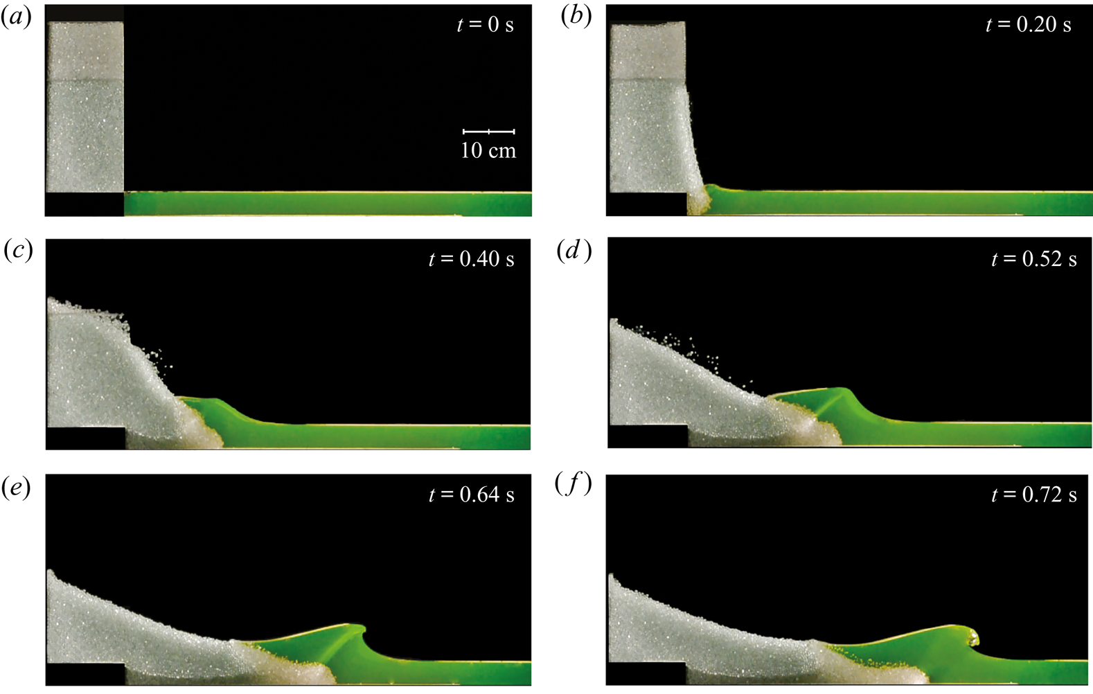
When a mass of rock or debris collapses into a body of water — a cliff face giving way into a fjord, a rockslide into a reservoir — the impact displaces the water and radiates an impulse wave outward, exactly as this granular column does when it crashes into the pool below it.

Laboratory experiments on exactly this configuration — a dry granular column released next to a shallow water layer — show that the collapsing grains act collectively like a moving piston: the wave amplitude relative to the water depth grows roughly linearly with the Froude number built from the granular front's horizontal velocity, essentially independently of the grain diameter and, more surprisingly, of the grain density. What sets the wave size is the volume of grains entering the water, not their mass — doubling the density barely changes the wave at all, while doubling the volume of the column does. Only a modest fraction of the column's initial potential energy, on the order of 10–20%, is ultimately transferred to the wave; most of it is dissipated within the granular flow itself before the grains ever reach the water.

The same physical mechanism, at a vastly larger scale, is behind some of the most destructive tsunamis on record — the specific wave regime reproduced in this case is classified in the Simulation Overview; MigFlow's own Lituya Bay case study on the Immersed Granular Flows axis explores one such historical event in more detail.

References & Sources

Simulated by

Simulation Overview

A granular column is held behind a thin vertical gate next to a shallow pool of fluid. Once the gate lifts, the column collapses under gravity and crashes into the pool, generating the impact wave described in the Real-world Phenomenon panel. Both phases use MigFlow's usual two-way PFEM–DEM coupling described in the Key Concepts above: the fluid mesh tracks the deforming free surface via PFEM, while the grains are resolved individually with NSCD contacts and coupled back to the fluid through the same VANS-family terms used elsewhere on this axis.

The gate itself is modelled as a moving rigid body inside the contact solver — frictionless against the grains so it can slide free — and its motion also drives the remeshing of the solid region behind it, so the fluid mesh, the free surface, and the granular column all update consistently at every step as the gate opens. This is one of the two validation benchmarks of Leyssens et al. (2025), set up to reproduce the experiments of Sarlin et al. (2021) on the nonlinear regimes of impulse waves generated by a granular collapse.

Sarlin et al. classify the resulting wave from the front's Froude number $\mathrm{Fr}_f = v_{fm}/\sqrt{gh_0}$, built from the granular front's maximum horizontal velocity $v_{fm}$ rather than a simple free-fall estimate, since it is the horizontal push of the grains — not their vertical fall — that drives the wave: a nonlinear transition wave below $\mathrm{Fr}_f\approx0.35$, a solitary non-breaking wave up to $\mathrm{Fr}_f\approx0.87$, and a transient bore beyond that. The configuration shown here matches the first of the paper's three validation cases, with $\mathrm{Fr}_f \approx 0.27$ (against $0.19$ measured experimentally) placing it in the nonlinear-transition-wave regime.

Key Parameters

Geometry

Domain (L × H) $2.0\times1.0\ \mathrm{m}$

Initial Column (Width × Height) $L_0\times H_0 = 0.145\times0.39\ \mathrm{m}$

Initial Fluid Depth $h_0 = 0.04\ \mathrm{m}$

Gate Opening Velocity $u_{\mathrm{gate}} = 1\ \mathrm{m/s}$ released after a $0.03\ \mathrm{s}$ settling time

Fluid & Grains

Fluid Density / Viscosity $\rho = 1000\ \mathrm{kg/m^3}$, $\eta = 10^{-3}\ \mathrm{Pa\cdot s}$ water

Surface Tension $\sigma = 7.28\times10^{-3}\ \mathrm{N/m}$

Grain Diameter / Density $d = 5\ \mathrm{mm}$, $\rho_p = 2500\ \mathrm{kg/m^3}$ polydisperse, ratio 1.2

Number of Grains $\approx 3400$

Grain–Grain / Grain–Wall Friction $\mu = 0.9$ / $0.9$

Grain–Gate Friction $\mu = 0$ gate slides freely past the grains

Wave Regime

Front Froude Number (PFEM-DEM) $\mathrm{Fr}_f \approx 0.27$ experimental: $0.19$

Wave Type nonlinear transition wave

Numerical

CFL Number $0.1$ adaptive time step

Final Time $1.03\ \mathrm{s}$

Featured Simulation · Multiphase PFEM

Three-Phase Rayleigh–Taylor Instability

Supplementary documentation

Ruyffelaere et al. (2026), preprint

Three stratified phases of densities $\rho = 1$ (bottom), $2$ (middle) and $4$ (top). Both interfaces stay sharp mesh edges throughout the mixing.

Simulated by

Simulation Overview

Three immiscible fluids are stacked with the heaviest on top and both interfaces slightly perturbed: gravity alone triggers the Rayleigh–Taylor instability. No surface tension, uniform kinematic viscosity, and a mesh rebuilt at every step from the advected nodes — the second validation benchmark of the multiphase PFEM framework.

The case exercises the remeshing itself. Both interfaces are recovered as edges of the new Delaunay triangulation through the protecting-ball criterion, and the topology is preserved down to $w_{\min}$, independently of the baseline interface resolution $s_{\min}$. Nodes are clustered around the interfaces only — a few thousand early on, against a uniform $h = 1/300$ grid for the reference computation — but the count climbs to about $2.5\times10^{5}$ once thin filaments permeate the whole domain.

Key Parameters

Geometry

Domain $\Omega = [0, H] \times [0, 3H]$ characteristic length $H = 1\ \mathrm{m}$

Initial interfaces $\Gamma_{1/2} = 1 + 0.1\cos(2\pi x)$, $\Gamma_{2/3} = 2 + 0.1\cos(2\pi x)$

Fluid Properties

Densities (bottom / middle / top) $\rho_1, \rho_2, \rho_3 = 1, 2, 4\ \mathrm{kg/m^3}$

Kinematic viscosity $\nu = 0.01\ \mathrm{m^2/s}$ uniform across the three phases

Interfacial surface tension $\gamma_{1/2} = \gamma_{2/3} = 0\ \mathrm{N/m}$

Gravity $g = 17.64\ \mathrm{m/s^2}$

Numerical

Interface resolution $s_{\min} = 1/83$ reference VOF grid: uniform $h = 1/300$

Topology threshold $w_{\min} = 1/830$

Number of nodes $2\,941 \rightarrow 249\,075$ from $t = 0.375$ to $t = 2$

Runtime $\approx 9\ \mathrm{min}$ single Intel Core Ultra 7 265H machine

Result & Validation

The minimum and maximum vertical positions of the dense and light phases fall between the two solvers reported by Garoosi et al. — an enhanced Volume-of-Fluid scheme and a Lagrangian MPS method — over the whole simulation.

This case is also the profiling reference for the method: about $48\%$ of an iteration goes into the linear solve, $38\%$ into the finite element assembly and $14\%$ into the meshing stage. The remeshing overhead stays moderate, and is largely offset by the reduction in degrees of freedom.

Real-world Phenomenon

Rayleigh–Taylor Mixing of Stratified Layers

A denser fluid resting on a lighter one releases its potential energy at the slightest disturbance: heavy spikes sink, light bubbles rise, and the shear rolls the fingers into mushroom heads. With three layers, the interfaces couple — the lower one is continuously deformed by the fingers falling through it — so both must be tracked at once.

The same instability shapes supernova remnants, volcanic plumes, inverted density layers in the ocean and the atmosphere, and any industrial pouring of liquids of different densities.

References & Sources

Featured Simulation · Multiphase PFEM

A Rigid Rotor Mixing Four Phases

Supplementary documentation

Ruyffelaere et al. (2026), preprint

Four fluid phases, one per quadrant, stirred by a four-bladed rigid rotor whose rotation is prescribed analytically.

Simulated by

Simulation Overview

A four-bladed rigid rotor stirs four fluid phases, one per quadrant. Its rotation is prescribed analytically and imposed on the fluid as a Dirichlet condition on the blade nodes, so the case is not a full fluid–structure solve: it isolates the geometric problem behind it, which is to keep a mesh conforming to a solid that sweeps across the entire domain.

The rotor boundary is treated exactly like a fluid–fluid interface — no manual remeshing around the blades, none of the distortion an ALE mesh suffers under large displacements, and no smearing of the solid surface over elements. The interior of the solid is meshed as well, so the same mesh could carry a structural solver for a fully coupled simulation, while the four phases are stretched into filaments preserved down to $w_{\min}$.

Key Parameters

Geometry

Domain (W × H) $1.0 \times 1.0\ \mathrm{m}$ no-slip on the four walls

Rotor blades (length × width) $0.5 \times 0.05\ \mathrm{m}$ two crossed blades, centred in the box

Fluid Properties

Densities (one per quadrant) $\rho \in \{1, 2, 3, 4\}\ \mathrm{kg/m^3}$

Kinematic viscosity $\nu = 0.01\ \mathrm{m^2/s}$ uniform, so $\mu = \rho\,\nu$ per phase

Surface tension $\sigma = 0\ \mathrm{N/m}$

Gravity $g = 9.81\ \mathrm{m/s^2}$

Rigid Body

Angular velocity $\omega = 10\ \mathrm{rad/s}$ prescribed, constant

Coupling Dirichlet on blade nodes solid interior meshed, ready for a structural solver

Numerical

Mesh size / interface resolution $h = 0.04\ \mathrm{m}$, $s_{\min} = 0.01\ \mathrm{m}$ topology threshold $w_{\min} = 0.002\ \mathrm{m}$

Time step / final time $\Delta t = 10^{-3}\ \mathrm{s}$, $t = 2\ \mathrm{s}$

Real-world Phenomenon

Stirring Immiscible Liquids with an Impeller

Blending liquids that do not mix on their own means forcing them through each other: an impeller stretches and folds the fluid, multiplying the interfacial area until diffusion or reaction can take over.

The same configuration appears in agitated tanks and rotor–stator mixers in the chemical, food and pharmaceutical industries, and wherever rotating machinery — turbines, pumps, agitators — interacts with the fluid it moves.

References & Sources

Featured Simulation · Multiphase PFEM

Two Colliding Jets

Supplementary documentation

Ruyffelaere et al. (2026), preprint

Two immiscible jets are injected from the left and right walls into a third, initially quiescent phase, and collide on the mid-plane.

Companion case with a single nozzle: the shear layer between the jet and the ambient phase rolls up into a train of vortices, each one still bounded by a sharp, conforming interface.

Simulated by

Simulation Overview

Two immiscible jets are issued from nozzles of different widths and velocities, cut in opposite lateral walls, into a third phase at rest; the collision front is therefore pushed towards the weaker jet, and the material leaves through the open top and bottom boundaries. Neither gravity nor surface tension is active: the case is about the boundary conditions.

An inlet is remarkably cheap to express in a Lagrangian framework. The inlet nodes are constrained to remain on the boundary, a parabolic profile is prescribed there, and the Lagrangian update advects the neighbouring material in exactly as it advects any interior node — no numerical flux, no convective term discretised at the boundary, and an unambiguous incoming phase. Mesh adaptation does the rest, inserting nodes as the injected material stretches away from the nozzle.

Key Parameters

Geometry

Domain (L × H) $2.0 \times 1.0\ \mathrm{m}$

Nozzle widths (left / right) $H/5$ / $H/10$ both centred at mid-height

Boundary Conditions

Inlet velocities (peak) $\mathbf{U}_l = [2, 0]^T$, $\mathbf{U}_r = [-1, 0]^T\ \mathrm{m/s}$ parabolic profile over each nozzle

Top & bottom boundaries open, $p = 0$ no-slip on the lateral walls, interrupted at the nozzles

Fluid Properties

Ambient phase $(\rho, \mu)$ $(0.1,\ 5\times10^{-4})$

Left / right jet $(\rho, \mu)$ $(1,\ 10^{-4})$ / $(2,\ 10^{-3})$

Surface tension $\sigma = 0\ \mathrm{N/m}$

Gravity $g = 0\ \mathrm{m/s^2}$

Numerical

Mesh size / interface resolution $h = 0.07\ \mathrm{m}$, $s_{\min} = 0.007\ \mathrm{m}$ topology threshold $w_{\min} = 1.4\times10^{-3}\ \mathrm{m}$

Time step / final time $\Delta t = 10^{-3}\ \mathrm{s}$, $t = 10\ \mathrm{s}$

Open Boundaries: an Honest Limitation

At low viscosity, the high-vorticity structures are eventually convected onto the open boundaries, where the normal velocity reverses locally and material re-enters the domain. Which phase enters is not determined by the data available to the solver: it is a modelling choice rather than a computed result.

The indetermination comes from the open-boundary model itself, not from the Lagrangian description — interface-capturing methods meet it in identical form — and treating it properly is a research question of its own.

Real-world Phenomenon

Impinging-Jet Mixing

Shooting two streams straight at each other is one of the fastest ways to mix them: their kinetic energy is dissipated in a small impingement zone that tears both into thin lamellae within milliseconds. When their momentum fluxes differ, as here, the stagnation plane shifts towards the weaker one.

Confined impinging jets are used wherever two reactive liquids must meet faster than they react: reaction injection moulding, nanoparticle precipitation, rocket and diesel injectors.

References & Sources

[1] Ruyffelaere, F., Henry, M., Lambrechts, J. & Remacle, J.-F. (2026). Topology-Preserving Mesh Adaptation for Sharp-Interface Multiphase PFEM. arXiv:2607.09446.

Featured Simulation · Multiphase PFEM–DEM

A Bubble and Grains

Supplementary documentation

Ruyffelaere et al. (2026), preprint Leyssens et al. (2025), J. Comput. Phys.

A gas bubble rises through a viscous liquid towards a raft of heavy grains floating just under the free surface, lifts it into a dome, and bursts.

Same configuration with a denser raft: the grains now load the interface enough to pierce the rising cap and split it into two separate bubbles.

Simulated by

Simulation Overview

Two fluid phases, a free surface and discrete grains denser than the liquid, all in the same simulation. A gas bubble released at the bottom of a viscous column rises towards a raft of grains floating just under the free surface: it flattens into a spherical cap, lifts the raft into a dome, drains the film beneath the surface and bursts through it, after which the grains settle back to the bottom.

Each grain is resolved individually by the NSCD contact solver, with friction against its neighbours and the walls, and coupled two-way to the flow through MigFlow's unresolved drag model — the PFEM–DEM coupling of Leyssens et al. (2025), here running on top of the multiphase remeshing. Surface tension is a membrane force built on the interface edges and balanced by duplicated pressure degrees of freedom rather than smeared over a band of elements, and the wall carries no surface energy, which keeps the contact lines at $90^\circ$.

The physical parameters below are those of the MigFlow dense-grain test case; the configuration in the video differs from it in the arrangement of the grains.

Key Parameters

Geometry

Domain (L × H) $1.0 \times 2.0\ \mathrm{m}$ no-slip top and bottom, free-slip side walls

Bubble radius / release point $R = 0.125\ \mathrm{m}$ at $(0.5,\ 0.25)$ free surface at $y = 1.2\ \mathrm{m}$

Fluid Properties

Liquid $(\rho, \mu)$ $(1000\ \mathrm{kg/m^3},\ 10\ \mathrm{Pa\cdot s})$

Gas $(\rho, \mu)$ $(1\ \mathrm{kg/m^3},\ 0.1\ \mathrm{Pa\cdot s})$ density ratio $10^3$, viscosity ratio $10^2$

Surface tension $\sigma = 24.5\ \mathrm{N/m}$ zero wall energy, contact lines at $90^\circ$

Gravity $g = 9.81\ \mathrm{m/s^2}$

Grains

Radius / density $r = 0.01\ \mathrm{m}$, $\rho_p = 5000\ \mathrm{kg/m^3}$ five times denser than the liquid

Friction (grain–grain / grain–wall) $\mu_f = 0.3$ NSCD contacts, two-way coupled to the flow

Numerical

Mesh size / interface resolution $h = 0.07\ \mathrm{m}$, $s_{\min} = 0.014\ \mathrm{m}$ topology threshold $w_{\min} = 0.007\ \mathrm{m}$

Time step / final time $\Delta t = 10^{-3}\ \mathrm{s}$, $t = 3\ \mathrm{s}$ direct linear solves with PARDISO

Real-world Phenomenon

Bubbles Bursting Through a Particle-Laden Surface

Grains that reach a liquid–gas interface are held there by capillarity even when far denser than the liquid, forming a raft that behaves like an elastic skin. A bubble arriving from below lifts that skin and either bursts through it, ejecting the grains, or — if the raft is dense enough — is pierced and split by them.

The same mechanisms drive froth flotation, particle-stabilised foams, the degassing of crystal-bearing magma, and the sea-spray aerosols produced when bubbles burst at the ocean surface.

References & Sources

Featured Simulation · Marker-based X-Mesh

Rayleigh–Taylor Instability

Supplementary documentation

He, Chen & Zhang (1999), J. Comput. Phys.

Evolution of the phase interface and close-up views of the fitted mesh as thin structures develop.

Simulated by

Simulation Overview

This classical two-dimensional benchmark places a heavy fluid above a light fluid in a vertical channel. A small sinusoidal perturbation triggers the instability, producing a descending heavy-fluid spike, a rising light-fluid bubble, and progressively rolled-up lateral structures. The explicit marker chain transports the sharp interface, while X-Mesh deforms a fixed-connectivity finite-element mesh so that selected edges remain fitted to it without remeshing.

The case tests the ability of the method to retain long, thin interfacial filaments and to introduce topology changes through a controlled feature-size criterion instead of numerical diffusion.

Key Parameters

Geometry

Domain $W \times 4W$

Initial perturbation $0.1\,W$

Flow Regime

Atwood number $A_t = 0.5$

Reynolds number $Re = 256$

Numerical

Boundary conditions Free slip

Mesh size $h = 0.0125\,W$

Result & Validation

The global morphology, symmetry, and penetration dynamics agree qualitatively with the reference results of He et al. Thin rolled-up structures remain sharply represented by locally anisotropic and nearly degenerated elements, even when their width falls below the characteristic background mesh size.

References & Sources

[1] A. Quiriny et al., Two-phase flow simulations using X-Mesh and an explicit marker interface representation, manuscript in preparation.
[2] X. He, S. Chen and R. Zhang, Journal of Computational Physics 152 (1999), 642–663.

Featured Simulation · Marker-based X-Mesh

Static Sessile Drops

Supplementary documentation

Relaxation of three sessile drops toward imposed Young angles of 60°, 90°, and 120°.

Simulated by

Simulation Overview

Three initially semicircular drops relax on a horizontal solid wall toward prescribed equilibrium contact angles. The marker representation explicitly tracks the two fluid–fluid–solid triple points of each drop, while the X-Mesh deformation keeps them attached to mesh vertices as they move tangentially along the wall.

Surface tension is introduced through a variational membrane and Young's law through a wall-energy term. This energy-based formulation recovers both acute and obtuse contact angles without curvature reconstruction or a special force at the triple point.

Key Parameters

Geometry

Domain $2 \times 1$

Initial drop radius $R = 0.3$

Fluid Properties

Density $\rho_1 = \rho_2 = 1$

Dynamic viscosity $\mu_1 = \mu_2 = 0.1$

Interface

Surface tension $\sigma = 1$

Young angles $60^\circ, 90^\circ, 120^\circ$

Numerical

Mesh size $h = 0.025$

Time step / final time $\Delta t = 7.8848\times10^{-4}$, $t = 3.1539$

Result & Validation

The final measured angles are 60.0356°, 90.0070°, and 119.9707°. The absolute error remains below 0.036°, demonstrating that the same formulation accurately preserves neutral, wetting, and non-wetting equilibrium configurations.

References & Sources

[1] A. Quiriny et al., Two-phase flow simulations using X-Mesh and an explicit marker interface representation, manuscript in preparation.

Featured Simulation · Marker-based X-Mesh

Capillary Rise

Supplementary documentation

Gründing et al. (2020), Appl. Math. Modelling

Transient rise, overshoot, and damped relaxation of the meniscus toward its hydrostatic equilibrium height.

Simulated by

Simulation Overview

This wetting benchmark follows the rise of a liquid meniscus in a narrow vertical channel. Symmetry reduces the computation to the right half-channel, bounded by a symmetry plane and a wetting wall. The explicit marker interface terminates at a moving triple point that is carried along the wall while the fitted mesh continuously conforms to the meniscus.

The simulation captures the initial rise and overshoot followed by damped oscillations toward hydrostatic equilibrium. It tests the coupled membrane and Young wall-energy formulation in a dynamic configuration with gravity and surface tension.

Key Parameters

Geometry

Half-gap / channel height $5\ \mathrm{mm} / 40\ \mathrm{mm}$

Young angle $\theta_Y = 30^\circ$

Fluid Properties

Liquid / gas density $83.1 / 0.0831\ \mathrm{kg/m^3}$

Dynamic viscosities $\mu_l = \mu_g = 10^{-2}\ \mathrm{Pa\cdot s}$

Physical Parameters

Surface tension $\sigma = 0.04\ \mathrm{N/m}$

Gravity $g = 4.17\ \mathrm{m/s^2}$

Numerical

Mesh size $h = 0.5\ \mathrm{mm}$

Time step / final time $\Delta t = 10^{-4}\ \mathrm{s}$, $t = 2.5\ \mathrm{s}$

Result & Validation

The computed final apex height is 19.3174 mm, compared with the corrected static value of 19.1538 mm, giving a relative error of 0.854%. The final contact angle is 30.1284°, showing that the formulation sustains the hydrostatic meniscus while retaining the prescribed triple-point condition.

References & Sources

[1] A. Quiriny et al., Two-phase flow simulations using X-Mesh and an explicit marker interface representation, manuscript in preparation.
[2] D. Gründing et al., Applied Mathematical Modelling 86 (2020), 142–165.

Featured Simulation · Marker-based X-Mesh

Model Name

Supplementary documentation

Poster name

Simulated by

Simulation Overview

Paragraph describing the numerical method, solver, and physical modeling choices used in the simulation: governing equations, discretisation approach, constitutive laws, and any notable numerical technique (remeshing, coupling scheme, etc.).

Key Parameters

Group title

Parameter name value = X unit

Real-world Phenomenon

Phenomenon name

Short paragraph explaining the physical mechanism behind the phenomenon.

Short paragraph giving further detail or a secondary mechanism.

Short paragraph noting the conditions under which the phenomenon occurs.