Immersed Granular Flows
Immersed Granular Flows is the applied face of MigFlow: the same grain solver (NSCD) and fluid solver (VANS), now put to work on what a granular medium actually does once a fluid moves through it. A dry pile of sand and a fluidised bed obey the same contact laws, but couple to wildly different physics — this axis is about the regimes, forces, and collective behaviours that emerge from that coupling, and the range of natural and industrial phenomena the framework can now represent as a result.
Key Concepts & Methodology
One Framework, Many Contexts
The same coupled NSCD–VANS machinery is deployed very differently depending on the problem. At the unresolved end, it homogenises industrial-scale configurations — fluidised beds, mixers, silos — where a coarse mesh spans many grains at once. At the fully resolved end, it captures the detailed wake of a single settling body. And coupled to PFEM's free-surface tracking, the same grain-contact solver extends beyond a fixed container altogether, to open, strongly deforming domains: a granular column crashing into a shallow pool, or a hillside collapsing into a lake.
Benchmark Before Belief
None of these contexts are trusted outright. Every configuration is first checked against a canonical, controlled benchmark before being pushed toward a real, uncontrolled event: a single settling cylinder validated by matching not just its mean fall speed but the wavelength and frequency of its wake-induced oscillations against a numerical reference; a granular column collapse validated against the measured runout and scaling law of a laboratory experiment. Only once a case reproduces this kind of quantitative benchmark is the same solver redeployed on a scenario — such as a historical landslide-tsunami — that can never be independently re-run in a lab.
Stokes Cloud: A Falling Swarm of Grains
Supplementary documentation
Simulation Overview
A compact, roughly spherical swarm of grains — a "Stokes cloud" — is released from rest in a viscous fluid and left to fall under gravity alone in a fully three-dimensional domain. This is the unresolved CFD-DEM model at its most classical: grains are solved individually with NSCD contacts, the fluid is solved on a coarser mesh with a stabilised P1-P1 finite element scheme (a pressure-Laplacian term keeps the equal-order velocity–pressure pair well-posed), and the two are coupled through a Dallavalle-type drag law corrected by a Wen & Yu porosity function, evaluated with the same semi-implicit scheme used elsewhere on this axis to keep the momentum exchange stable. The fluid mesh is periodically rebuilt and refined tightly around the grains' current position as the cloud moves, so resolution follows the swarm rather than being fixed in space.
As the cloud falls, it drives its own circulating flow: fluid streamlines close around it, elongating the upper part while the lower part flattens. Grains at the rear continually leak out of this closed envelope into a growing trailing tail — the leakage rate set by the cloud's falling speed, its radius, and the grain radius — until the depleted core lets fluid punch straight through, turning the swarm into an open torus that goes on to break into one or more secondary droplets. This configuration releases two clouds with a diagonal offset, reproducing the interacting-cloud case of Constant et al. (2018).
Key Parameters
Cloud & Grains
Fluid & Regime
Geometry & Numerical
Sedimenting Particle Clouds
A swarm of small particles released together in a fluid does not settle as a diffuse haze: the grains drag fluid down with them, and the resulting collective flow holds the swarm together as a coherent, falling cloud — a self-organised behaviour quite different from how a single isolated grain settles.
This kind of collective settling shows up whenever fine particulate matter is released into a fluid: sediment or ash plumes settling through water or air, powders and reagents injected into industrial mixing or chemical processes, and dense suspensions such as concrete, cement pastes, or agro-food and pharmaceutical formulations. Understanding how such a cloud stretches, sheds a trailing tail, and eventually breaks apart is central to predicting how far and how fast the material spreads before it settles out.
Avalanche Clusters
Supplementary documentation
Granular Avalanches & Grain Shape
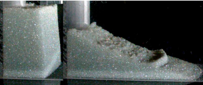
The collapse of a granular column — released from a confined pile and left to spread under its own weight — is a standard laboratory stand-in for avalanches, debris flows, and landslides. How far the resulting deposit travels, its runout, follows a power law in the column's initial aspect ratio, largely independent of grain size, and consistently reduced by the presence of a surrounding fluid.
Most of that phenomenology has been established for round grains, but few natural or industrial grains are actually spherical. Elongated grains — driftwood debris jamming at a bridge, or the layered fragments produced by a pyroclastic or debris flow — can align with the flow, interlock, and jam in ways a disc never does, changing how the moving mass channels its energy even when the overall runout law stays the same.
Simulation Overview
The collapse of a granular column is a classic benchmark for immersed granular flows, but here the grains themselves are not disks: each is a rigid line-cluster of 3–4 bonded disks, giving the assembly an orientation that can align, cluster, and jam in ways a circular grain never can. The solid phase is solved with NSCD exactly as elsewhere on this axis; what differs is that the fluid–grain interaction is computed disk by disk and then summed into a single net force and torque on the elongated grain, so that its own rotation naturally emerges from the drag imbalance across its length.
The fluid is solved on a coarser mesh through the same unresolved, porosity-averaged formulation used across the group,
with $\phi$ the porosity and $\mathbf{v}$ the volume-averaged fluid velocity, coupled semi-implicitly to the grains for stability. At each disk, the interaction force combines the pressure gradient with a Dallavalle-type drag corrected for the local porosity (Wen & Yu),
Columns spanning aspect ratios $H_0/L_0$ from 0.125 to 16, dry or immersed, and with either randomly oriented or pre-aligned grains, are released and left to collapse. Across the whole set, the final runout collapses onto a single scaling law driven by the front's kinetic energy at the moment it detaches — grain elongation shifts the prefactor of that law, but not its exponent, meaning shape changes how far a granular avalanche can travel without changing the fundamental physics that governs it.
Key Parameters
Grain Properties
Friction & Fluid
Geometry & Numerical
Lituya Bay Landslide-Tsunami
Supplementary documentation
The 1958 Lituya Bay Megatsunami
On July 10, 1958, a magnitude 8.3 earthquake on the Fairweather Fault triggered a major subaerial landslide into Gilbert Inlet, at the head of Lituya Bay, Alaska. The landslide struck the water at high speed, generating the highest wave run-up ever recorded: 524 metres, stripping trees and soil down to bedrock on the opposing hillside far above the shoreline.
It remains one of the best-documented case studies of a subaerial landslide tsunami, and a natural stress test for the same PFEM–DEM coupling introduced above: a real, historical event with an independently estimated slide mass and a measured run-up, reconstructed here from first principles rather than fitted to it.
The simulation reproduces this strikingly well: a thin layer of water is tracked reaching as high as 750 m on the opposite shore — an overestimate, since it assumes the water slides freely along the boundary — but already at 500 m the water retains enough inertia to cause damage, closely matching the 524 m run-up actually observed in 1958.
References & Sources
- [1] Fritz, H.M., Mohammed, F. & Yoo, J. (2009). Lituya Bay landslide impact generated mega-tsunami 50th anniversary. Pure and Applied Geophysics, 166, 153–175.
- [2] Leyssens, T., Henry, M., Lambrechts, J., Legat, V. & Remacle, J.-F. (2025). A coupled PFEM-DEM model for fluid-granular flows with free surface dynamics applied to landslides. Journal of Computational Physics, 537, 114082.
Simulation Overview
The bay's cross-section is reconstructed as an inclined slope descending into a water-filled basin, with the rock mass represented as a population of large, rigid grains resolved individually by NSCD. The fluid is tracked with the same two-way PFEM–DEM coupling introduced in the Key Concepts above: the mesh is entirely rebuilt from an alpha-shape at every step and advected with the fluid's own velocity, so the free surface can deform without limit as the slide crashes in and the resulting wave races across the bay.
Because the slide is modelled with a comparatively small number of large grains rather than a grain-for-grain reconstruction of the real rockfall, a volume correction factor rescales their density so that the simulated mass matches the historical estimate of the slide directly — keeping the momentum delivered to the water physically consistent with the real event, even though the granular representation itself is necessarily coarse.
Based on wave-type analysis and the front Froude number, the resulting wave is expected to behave as a bore, and the simulation confirms it: the wave does not have time to break before crossing the bay and hitting the opposite shore, where it reflects and produces a secondary sloshing wave of smaller amplitude. Comparing the tracked wave amplitude at a point 885 m from the initial shoreline against recorded data, the Lagrangian formulation captures the main trends of the wave dynamics well. Displaced rocks settle throughout the bay, with the largest deposits forming near the impact zone and near the opposite shore.
Key Parameters
Bay Geometry
Materials
Numerical
Validation
Cylinder Sedimentation
Supplementary documentation
Simulation Overview
This case validates the two-way fluid–grain coupling at the fully resolved end of the axis: a rigid 2D cylinder is released from rest in a quiescent viscous fluid and left to fall under gravity, with the mesh refined enough to resolve the boundary layer directly around it (roughly 8 elements across its diameter), rather than reconstructing it through a drag correlation. Results are compared directly against the reference numerical study of Namkoong et al.
With a solid-to-fluid density ratio of only 1.01, the cylinder is close to neutrally buoyant, so its descent is gentle enough for the wake dynamics — rather than gravity alone — to dominate its trajectory. As it accelerates, vortex shedding sets in and begins to modulate the fall.
The streamwise velocity initially overshoots the terminal velocity $U_t$, then is damped down as shedding becomes established; the lateral velocity oscillates with an opposite-sign pattern, its direction set by small mesh-induced asymmetries. Both the wavelength and frequency of these oscillations match the reference closely, confirming that the coupling captures not just the mean settling speed but the full unsteady, wake-driven dynamics of the descent.
Key Parameters
Cylinder & Fluid
Flow Regime
Geometry & Numerical
Sedimenting Bodies & Wake-Induced Oscillations
A body released from rest in a viscous fluid rarely falls in a straight line at constant speed. As it accelerates, it sheds vortices into its wake; the resulting asymmetric pressure field pushes it sideways and modulates its fall speed, producing the oscillatory, zig-zagging descent seen throughout sedimentation experiments and industrial particle-settling processes.
This same wake–body interaction is the building block for richer collective behaviour — it is what drives the drafting–kissing–tumbling dynamics between two settling particles, and more broadly governs sediment transport and particle classification wherever bodies fall through a fluid.